Medical Imaging using Fastai
Reviewing fastai notebook 60_medical.imaging.ipynb


- Patching
- Class TensorDicom
- Class PILDicom
- >> Side Note: Pixel Distribution
- >> Side Note: Windowing
- show
60_medical_imaging which can be found here
Import the libraries
from fastai.basics import *
from fastai.vision.all import *
from fastai.data.transforms import *
from fastai.medical.imaging import *

import pydicom,kornia,skimage

try:
    import cv2
    cv2.setNumThreads(0)
except: pass

import seaborn as sns
sns.set(style="whitegrid")
sns.set_context("paper")
#Load the Data
pneumothorax_source = untar_data(URLs.SIIM_SMALL)
Provides a convenient way of recursively loading .dcm images from a folder. By default the folders option is set to False but you could specify a specific folder if required
#get dicom files
items = get_dicom_files(pneumothorax_source, recurse=True, folders='train')
items
Pydicom is a python package for parsing DICOM files and makes it easy to covert DICOM files into pythonic structures for easier manipulation. Files are opened using pydicom.dcmread
img = items[10]
dimg = dcmread(img)
type(dimg)
You can now view all the information within the DICOM file. Explanation of each element is beyond the scope of this tutorial but this site has some excellent information about each of the entries. Information is listed by the DICOM tag (eg: 0008, 0005) or DICOM keyword (eg: Specific Character Set)
dimg
Some key pointers on the tag information above:
- Pixel Data (7fe0 0010) - This is where the raw pixel data is stored. The order of pixels encoded for each image plane is left to right, top to bottom, i.e., the upper left pixel (labeled 1,1) is encoded first
- Photometric Interpretation (0028, 0004) - aka color space. In this case it is MONOCHROME2 where pixel data is represented as a single monochrome image plane where low values=dark, high values=bright. If the colorspace was MONOCHROME then the low values=bright and high values=dark info.
- Samples per Pixel (0028, 0002) - This should be 1 as this image is monochrome. This value would be 3 if the color space was RGB for example
- Bits Stored (0028 0101) - Number of bits stored for each pixel sample
- Pixel Represenation (0028 0103) - can either be unsigned(0) or signed(1). The default is unsigned. This Kaggle notebook by Jeremy explains why BitsStored and PixelRepresentation are important
- Lossy Image Compression (0028 2110) - 00 image has not been subjected to lossy compression. 01 image has been subjected to lossy compression.
- Lossy Image Compression Method (0028 2114) - states the type of lossy compression used (in this case JPEG Lossy Compression)
- Pixel Data (7fe0, 0010) - Array of 118256 elements represents the image pixel data that pydicom uses to convert the pixel data into an image.
Important tags not included in this dataset:
- Rescale Intercept (0028, 1052) - The value b in relationship between stored values (SV) and the output units. Output units = m*SV + b.
- Rescale Slope (0028, 1053) - m in the equation specified by Rescale Intercept (0028,1052).
The Rescale Intercept and Rescale Slope are applied to transform the pixel values of the image into values that are meaningful to the application. These two values allows for transforming pixel values into Hounsfield Units(HU). Densities of different tissues on CT scans are measured in HUs
The Hounsfield scale is a quantitative scale for describing radiodensity in medical CT and provides an accurate density for the type of tissue. On the Hounsfield scale, air is represented by a value of −1000 (black on the grey scale) and bone between +300 (cancellous bone) to +3000 (dense bone) (white on the grey scale), water has a value of 0 HUs and metals have a much higher HU range +2000 HUs.
The pixel values in the histogram above do not correctly correspond to tissue densities. For example most of the pixels are between pixel values 0 and 200 which correspond to water but this image is predominantly showing the lungs which are filled with air. Air on the Hounsfield scale is -1000 HUs.
This is where RescaleIntercept and RescaleSlope are important. Fastai provides a convenient way by using a function scaled_px to rescale the pixels with respect to RescaleIntercept and RescaleSlope.
rescaled pixel = pixel * RescaleSlope + RescaleIntercept
By default pydicom reads pixel data as the raw bytes found in the file and typically PixelData is often not immediately useful as data may be stored in a variety of different ways:
- The pixel values may be signed or unsigned integers, or floats
- There may be multiple image frames
- There may be multiple planes per frame (i.e. RGB) and the order of the pixels may be different These are only a few examples and more information can be found on the pycidom website
What does pixel data look like?
dimg.PixelData[:200]
Because of the complexity in interpreting PixelData, pydicom provides an easy way to get it in a convenient form: pixel_array which returns a numpy.ndarray containing the pixel data:
dimg.pixel_array, dimg.pixel_array.shape
Inherits from TensorImage and converts the pixel_array into a TensorDicom
ten_img = TensorDicom(dimg.pixel_array)
ten_img
TensorDicom uses gray as the cmap default so when you view the image using the show function:
ten_img.show()

However this can be changed to the bone cmap which is better at differentiating different areas of the image.
class TensorDicom(TensorImage): _show_args = {'cmap':'bone'}
ten_img2 = TensorDicom(dimg.pixel_array)
ten_img2.show()

matplotlib.rcParams which in this case sets the cmap values to bone
matplotlib.rcParams['image.cmap'] = 'bone'
Inherits from PILBase
Opens a DICOM file from path fn or bytes fn and load it as a PIL Image. The DICOM is opened using pydicom.dcmread and accesses the pixel_array and returns the full size of the image.
type(PILDicom.create(img))
PILDicom.create(img)

Converts the pixel_array into a tensor
pixels(dimg)
pixels scaled by RescaleSlope and RescaleIntercept. The slim SIIM_SMALL dataset does not have RescaleSlope (0028,1053) or RescaleIntercept (0028,1052) in the dataset.
To illustrate the importance of RescaleSlope and RescaleIntercept, I am going to use an image from this dataset which has a:
- RescaleIntercept of
-1024 - RescaleSlope of
1
test_i = 'D:/Datasets/train_test/167.dcm'
test_im = dcmread(test_i)
timg = PILDicom.create(test_i)
timg.show()

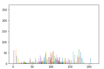
We can then plot a histogram to represent the pixel values within the dicom image
px = test_im.pixels.flatten()
plt.hist(px, color='c')

The image above is a slice of the chest cavity that predominantly consists of air(dark areas) and there is not much bone(bright white areas) in the picture but the histogram shows that the bulk of the pixels are distributed around 0 and 1000 which does not correctly represent the tissues densities in the image.
This why RescaleSlope and RescaleIntercept are important and scaled_px uses these values to correctly scale the image so that they represent the correct tissue densities.
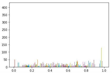
tensor_dicom_scaled = scaled_px(test_im) #convert into tensor taking RescaleIntercept and RescaleSlope into consideration
plt.hist(tensor_dicom_scaled.flatten(), color='c')

Having well scaled inputs is really important in getting good results from neural net training ref. This means having a normal or uniform distribution. The pixels in the DICOM image do not show a uniform distribution
#switching back to the SIIM dataset
px = dimg.pixels.flatten()
plt.hist(px, bins=50, color='g');

In this case the image is showing multimodal distribution(having more than 2 peaks). Another case could be where the distribution is bimodal(having 2 distinct peaks). The functions below provide a means of splitting the range of pixel values into groups so that each group has an equal number of pixels
This is a numpy based function to split the range of pixel values into groups, such that each group has around the same number of pixels
arry = array_freqhist_bins(dimg.pixel_array)
arry
Splits the range of pixel values into groups, such that each group has around the same number of pixels where the input is a tensor. You can create a tensor of the image by using pixels
tensor_dicom = pixels(dimg)
tensor_dicom
You can then specify the number of bins or groups you want to split the pixels into, the default is 100
t_bin = tensor_dicom.freqhist_bins(n_bins=100)
t_bin
freqhist_bins splits the pixels into bins, the number of bins set by n_bins. So for the above example:
freqhist_bins flattens out the image tensor (in this case 1024 by 1024 into a flattened tensor of size 1048576 (1024*1024)
- setting `n_bins` to 1 for example means it will be split into 3 bins (the beginning, the end and the number of bins specified by `n_bins`
- each bin is then scaled to values between 0 and 255 (in this case the bulk of pixels are grouped at 3, 103 and 203
with n_bin set to 1
t_bin = tensor_dicom.freqhist_bins(n_bins=1)
plt.hist(t_bin, bins=t_bin)

plt.hist(t_bin, bins=t_bin, color='c'); plt.plot(t_bin, torch.linspace(0,1,len(t_bin)));dimg.show(t_bin)


with n_bins of 100
t_bin = tensor_dicom.freqhist_bins(n_bins=100)
plt.hist(t_bin, bins=t_bin)

plt.hist(t_bin, bins=t_bin, color='c'); plt.plot(t_bin, torch.linspace(0,1,len(t_bin)));dimg.show(t_bin)


A way to scale a tensor of pixels evenly using freqhist_bins to values between 0 and 1.
tensor_dicom
The tensor has values between 0 and 255
#Run to view - commented out to reduce file size
#plt.hist(tensor_dicom, bins=100)
The above commented out code displays a histogram of pixel values which range from 0 to 255
Using hist_scaled gets values now scaled between 0 and 1
tensor_hists = tensor_dicom.hist_scaled()
tensor_hists
#plotting the scaled histogram
#plt.hist(tensor_hists, bins=100)
Scaled histogram now has pixel values ranging from 0 to 1
Similar to Tensor.hist_scaled except that the input here is a DcmDataset and you can set the minimum and maximum pixel values
dimg.pixel_array
data_scaled = dimg.hist_scaled(min_px=1, max_px=20)
data_scaled
#Using min_px = 1 and max_px = 20
plt.imshow(data_scaled, cmap=plt.cm.bone);

#Using min_px = 100 and max_px = 244
data_scaled2 = dimg.hist_scaled(min_px=100, max_px=244)
plt.imshow(data_scaled2, cmap=plt.cm.bone)

DICOM images can contain a high amount of voxel values and windowing can be thought of as a means of manipulating these values in order to change the apperance of the image so particular structures are highlighted. A window has 2 values:
l = window level or center aka brightness
w = window width or range aka contrast
Example: from here
Brain Matter window
l = 40 (window center) w = 80 (window width)
Voxels displayed range from 0 to 80
Calculating voxel values:
- lowest_visible_value = window_center - window_width / 2
- highest_visible_value = window_center + window_width / 2
(lowest_visible_value = 40 - (80/2), highest_visible_value = 40 + (80/2))
Takes 2 values w and l
fastai conveniently provides a range of window width and centers (dicom_windows) for viewing common body areas:
brain=(80,40),
subdural=(254,100),
stroke=(8,32),
brain_bone=(2800,600),
brain_soft=(375,40),
lungs=(1500,-600),
mediastinum=(350,50),
abdomen_soft=(400,50),
liver=(150,30),
spine_soft=(250,50),
spine_bone=(1800,400)plt.imshow(dimg.windowed(w=1500, l=-600), cmap=plt.cm.bone)

The above is the same as below using dicom_windows.lungs
plt.imshow(dimg.windowed(*dicom_windows.lungs), cmap=plt.cm.bone)
Example of how windowing works
img = items[10]
dimg = dcmread(img)
Convert a DICOM image into tensors
tensor_dicom = pixels(dimg)
tensor_dicom
View a portion of the image
portion = tensor(tensor_dicom)[200:440,600:840]
portion.shape
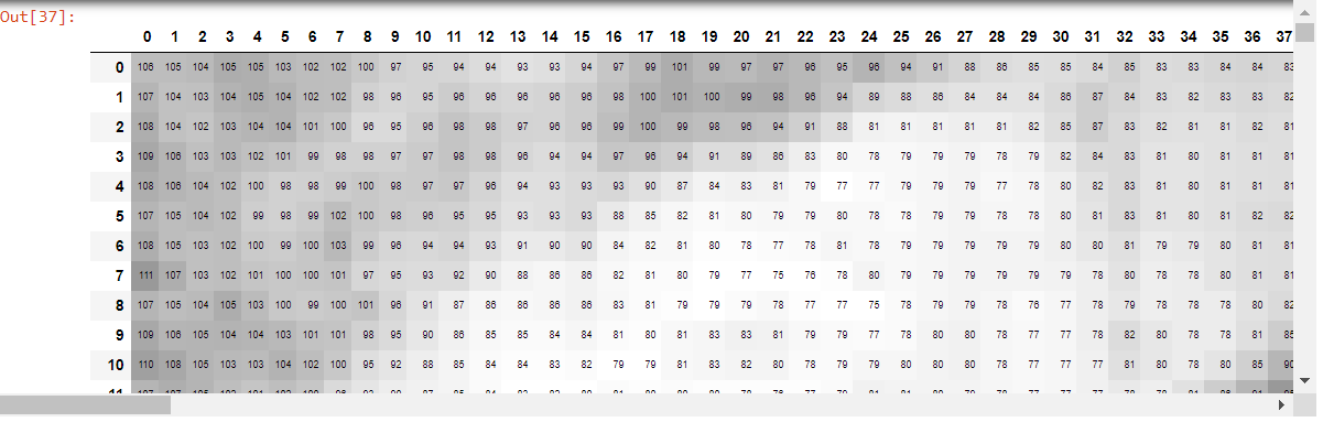
df = pd.DataFrame(portion)

#uncomment to run on locally
#df.style.set_properties(**{'font-size':'6pt'}).background_gradient('Greys')
The dataframe created by df looks like this:
You can create your own window parameters, here we create one named test_window
dicom_windows = types.SimpleNamespace(
    test_window=(50,60)
)
We can apply the test_window window to portion image
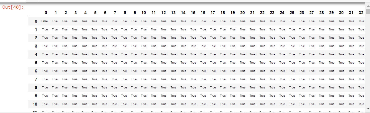
r = portion.windowed(w=50, l=60)
#This will produce a Dataframe of each pixel whether 'true' or 'false'
#uncomment to run locally

test_e = portion.mask_from_blur(dicom_windows.test_window, thresh=0.05, remove_max=True)
#dfe = pd.DataFrame(test_e)
#dfe.style.set_properties(**{'font-size':'6pt'}).background_gradient('Greys')
imk = [portion,r, test_e]
show_images(imk, titles=('orig', 'windowed', 'mask'), figsize=(15,15))

using show_images the images appear green because show_images and show_image by default use the 'viridis' colormap and PILBase follows the same default colormap. However we had earlier changed the Matplotlib.rcParams to bone
Inherits from show_image and is customized for displaying DICOM images
dimg.show(scale=True, cmap=plt.cm.bone, min_px=-1100, max_px=None, ax=None, figsize=(6,6), title='Test', ctx=None)

Jeremy mentioned in this article about using a 'rainbow colormap' to fully utilize our computer's ability to display color
dimg.show(cmap=plt.cm.gist_ncar, figsize=(6,6))

This class returns TensorImageBW
Inherits from PILBase
Gets the % of pixels within a window w, l
For example using lungs as the dicom_window (1500,-600) we see that 80% of the pixels are within the window
dimg.pct_in_window(*dicom_windows.lungs)
What about the test_window that was created:
dimg.pct_in_window(*dicom_windows.test_window)
A way of blurring the image uniformarly taking in 2 inputs: the input image and the scale of blurring
ims = dimg.hist_scaled(), uniform_blur2d(dimg.hist_scaled(),20), uniform_blur2d(dimg.hist_scaled(),50)
show_images(ims, titles=('original', 'blurred 20', 'blurred 50'), figsize=(15,15))

Uses gaussian_blur2d kornia filter
gims = dimg.hist_scaled(), gauss_blur2d(dimg.hist_scaled(),20), uniform_blur2d(dimg.hist_scaled(),50)
show_images(gims, titles=('original', 'gauss_blurred 20', 'gauss_blurred 50'), figsize=(15,15))

As explained in this notebook Jeremy uses these methods in cleaning the data in order to only retain information that is relevant. For example you use gauss_blur2d to blur the image and then select the areas that are bright
px = dimg.windowed(w=1100, l=-500)
show_image(px, figsize=(4,4));

blurred = gauss_blur2d(px, 125)
show_image(blurred, figsize=(4,4));

show_image(blurred>1, figsize=(4,4));

Function to create a mask from the blurred image that takes in the input and window, sigma and threshold values
#switching back to this image which allows the use of `scaled_px`
test_i = 'D:/Datasets/train_test/167.dcm'
test_im = dcmread(test_i)
timg = PILDicom.create(test_i)
timg.show()
mask = test_im.mask_from_blur(dicom_windows.lungs, sigma=0.1, thresh=0.75, remove_max=False)
wind = test_im.windowed(*dicom_windows.lungs)

_,ax = subplots(1,2)
show_image(wind, ax=ax[0])
show_image(mask, alpha=0.5, cmap=plt.cm.Reds, ax=ax[1]);

bbs = mask2bbox(mask)
lo,hi = bbs
show_image(wind[lo[0]:hi[0],lo[1]:hi[1]]);

show_images(dimg.to_nchan([dicom_windows.brain,dicom_windows.subdural,dicom_windows.abdomen_soft]))

show_images(dimg.to_nchan([dicom_windows.brain]))

Save a tensor into a .jpg with specified windows
tensor_dicom = pixels(dimg)
tensor_dicom.save_jpg(path=(pneumothorax_source/f'train/01tensor.jpg'), wins=[dicom_windows.lungs, dicom_windows.subdural])
show_image(Image.open(pneumothorax_source/f'train/01tensor.jpg'))

Save a DICOM image into a .jpg
dimg.save_jpg(path=(pneumothorax_source/f'train/01dicom.jpg'), wins=[dicom_windows.lungs, dicom_windows.lungs])
show_image(Image.open(pneumothorax_source/f'train/01dicom.jpg'))

Zoom's image by specifying pixel ratio
dimg2 = dcmread(items[11])
dimg2.zoom(0.1)
dimg2.show()

dimg2.zoom(0.5)
dimg2.show()

dimg2 = dcmread(items[11])
dimg2.shape, dimg2.show()

dimg2.zoom_to(90)
dimg2.shape, dimg2.show()
